Google Sheets is Google’s version of a spreadsheet as Excel is to Microsoft. The cloud-based spreadsheet app is robust and allows you to a lot of things. Many organisations and teams use it to organise data for more productivity. It can also be used for personal life like for keeping records of your finances and more.
As a business owner or HR manager, you will need to calculate the difference between two timestamps. One of your employee could come in at 8:30AM and leave at 5:00PM. You may need to calculate the duration between these times for record purposes. The duration for this two time period is 8 hours, 30 minutes. Google Spreadsheet cannot do this calculation directly and you’ll need to use certain parameters. In this guide, we’ll show you how this works:
How to Calculate Time in Google Sheets
You can easily measure the difference between two cells having time data, provided that the data is set correctly. If you input 8:00AM and 9:00AM without setting the right parameters to calculate the difference between then, Google Sheets will return a result of 100 rather than 60 minutes or 1 hour.
You’ll need to format the time columns as “Time” and the duration column as “Duration”
Also, you have to note that the calculation is always done backward (time out – time in).
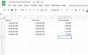
Below are the steps to make a formatted time sheet with columns that show the time people started work, the time they left, and the duration between these data:
1. Open the spreadsheet document.
2. Now, select your “Time In:’ column, and then click the “123” format drop-down.
3. From the drop-down, select “Time” as the format.
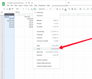
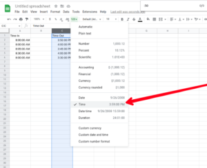
4. Select the “Time Out:” column, and then click the “124′ drop-down menu. From there select “Time”.
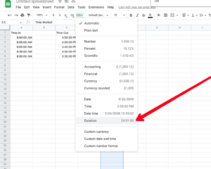
5. Now in the duration column which in your spreadsheet can be “Hours Worked”, click on the “123” drop-down menu, and select “Duration” as the format.
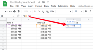
6. Now to the formula: go to the “Hours Worked” column and type the formula below:
=(C2-A2)
Where “C2” is the Time Out, and A2 is the Time In.
How to Add Time Gaps or Work Breaks When Calculating Time in Google Sheets
You can add time gaps to your sheet to account for for things like leaves and lunches. You may want to have a seperate column for this. Here’s how to do it:
1. Select your Break Out column and click the “123” format dropdown.
2. From the drop-down menu, select “Time” as the format.
3. Also in the Break In column, click on the “123” drop down.
4. Choose “Time” as the format.
5. You can then go ahead to calculate the hours for the “Hours Worked” column. Use the formula below:
=(C2-A2)+(E2-G2),
C2 represents Break Out
A2 represents Time In
E2 represente Time Out
G2 represents Break In
Rounding Up…
Google Sheets is a powerful application, no doubt. With the time functions, you don’t have to stress and do a lot of paper work or mathematical calculation in a bit to calculate the time your employees spend at work. The formula is simple and allows you to calculate time duration fast. We hope you found this helpful? If you did, kindly leave a comment and don’t forget to share…
Leave a Reply